
If you’re working on an Excel spreadsheet that you want to share or collaborate on with others, you might want to think about adding a watermark.
A watermark identifies you as the owner or creator of the spreadsheet, and usually incorporates your name or your business branding. It could be a logo, a signature, a photo, or other type of identifier.
If you want to know how to add a watermark in Excel, here’s what you’ll need to do.
Table of Contents
Creating a watermark image for Excel spreadsheets
Excel doesn’t have a watermark feature exactly, but all the steps you need to create a watermark are available. To add a watermark to an Excel spreadsheet, you’ll need to create an image that contains your branding using an outside tool.

As we’ve mentioned, this image could contain your name or signature, a logo, or other text, symbol, or identifier. Watermarks are usually small in size and are placed in areas of the spreadsheet that avoid conflicting with or distracting from the main content, such as the header or footer areas.
You may want to edit a photo to create a watermark to use in your spreadsheet. Alternatively, you could use tools like Paint, GIMP, or Photoshop to create a watermark image separately. Excel does have some basic drawing tools, but it doesn’t allow you to use them to create a watermark for your spreadsheet.
Once you’ve created a watermark outside of Excel, save it as a PNG or JPG file on your PC or Mac.
How to insert a watermark in Excel
Once you’ve created or sourced your watermark image, you’ll need to insert it into your Excel spreadsheet. Here’s how:
- Open your Excel spreadsheet and press View > Page Layout.If you’re using an older version of Excel, press Insert > Header & Footer instead.
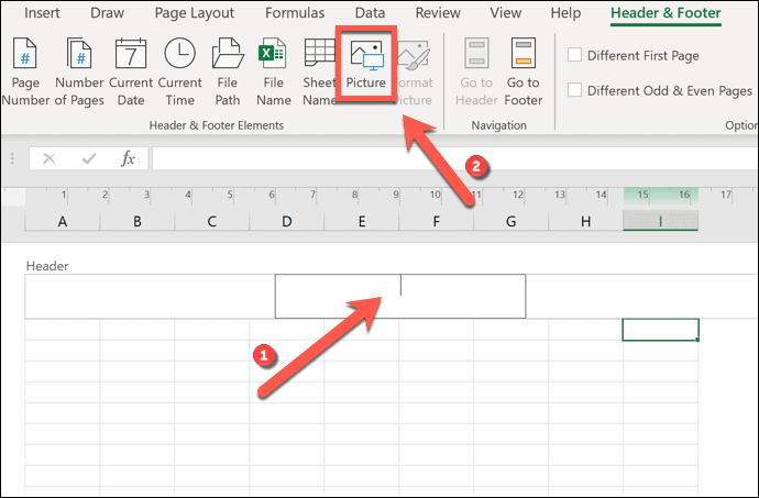
- Tap on the Add header (top) or Add footer (bottom) sections to edit them.
- In the Header & Footer ribbon bar tab, press Picture.
- In the Insert Pictures menu, press Browse to locate your file.
- Locate your watermark image and press Insert.
- Your image will appear as &[Picture], a text placeholder representing the final image.
- Select an area outside of the header or footer areas to view the watermark image.
Inserted watermark images will appear, full-sized, in the spreadsheet. If the original image is too big, the image will appear outside the boundaries of your header or footer. If this happens, you’ll need to format your image.
How to resize a watermark in Excel
Watermark images added to Excel headers and footers are inserted using the original image size and without any additional effects added. If you’d like to modify your watermark image, you’ll need to edit the image using the Format Picture menu.
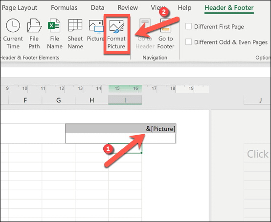
- Press View > Page Layout to access the header and footer areas, then select the &[Picture] placeholder text.
- In the Header & Footer ribbon bar tab, press Format Picture.
- To resize the image, lower or raise the values in the Height and Width sections.
- If you want to crop any areas of the image, press Picture and increase any of the values (in 0.1cm increments) in the Crop from section.
- If you want to make the image grayscale, black and white, or add a high-contrast washout effect, press Picture > Color and select one of the drop-down menu options.
- To save your changes, press OK. Tap outside of the header or footer areas to view the changes.
The watermark image you’ve added should appear on each virtual page in the Page Layout view. If you print your spreadsheet, the watermark will also appear on each page. The watermark won’t be visible in the standard Normal view as you edit, however.
Read Also: How to Divide in Excel